Inspired
by biological Neural Networks, in particular the functionality of the brain,
artificial Neural Networks are a branch of machine learning that uses
statistical algorithms to predict the outcomes of functions with multiple known
inputs. Neural Networks are usually represented as a system of interconnected “neurons”,
which are capable of pattern recognition and computing values. The formative
years of Artificial Neural Networks were from 1943 to 1958, where many large
and influential discoveries were made. In 1958, a famous researcher named Frank
Rosenblatt proposed that a “perceptron” could be used as the first model for
supervised machine learning.
A
perceptron is the simplest form of a neural network and is used to classify
patterns that are on opposite sides of a hyperplane, also known as linearly
separable patterns. A perceptron is made of a single neuron with customizable synaptic
weights. With his perceptron, Rosenblatt proved the perceptron convergence theorem which stated that if the vectors
used to train the perceptron were taken from two linearly separable classes,
then the algorithm will converge and positions the decision surface in the form
of a hyperplane between two classes.
Rosenblatt
made many public statements about the perceptron and it’s ability to learn,
thus sending the Artificial Intelligence community into heated debate. It was
later discovered that the single-layer perceptron could not be trained to
recognize many classes or patterns. This stalled the field of neural network
research considerably before people realized that a “feed-forward neural
network”, also known as a “multi-layer perceptron” that had two or more layers,
had much more processing power than previous models. It was then shown that
multi-layer perceptrons could solve even problems that were not linearly
separable like XOR. Single-layer perceptrons were only able to solve linearly separable
problems like AND and OR, and in 1969 two researchers named Marvin Minsky and
Seymour Papert wrote a book titled Perceptrons that proved that single-layer
perceptrons would never be able to learn non-linearly separable patterns like
XOR.
The
multi-layer perceptron computes a single output from multiple inputs by forming
a linear combination (propagation rule) according to its input weights and then
putting the output through a linear activation function. This can be
mathematically represented by:
Where
“w” represents the value of the weights, “x” is the value if the inputs, β is
the bias, and λ is the activation function. Although, in Rosenblatt’s original
multi-layer perceptron a Heaveside step function was used as the activation
function, in recent days a logistic sigmoid function is used as it is
mathematically convenient and is close to the origin and then moves quickly
when leaving the origin.
A
single-layer perceptron is not very useful, not only for the reasons stated
previously but also because of it’s limited mapping ability. Also, no matter
what activation function is used, the single-layer perceptron will always
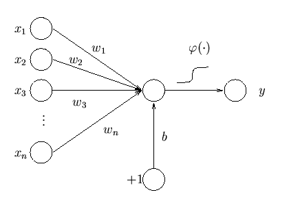
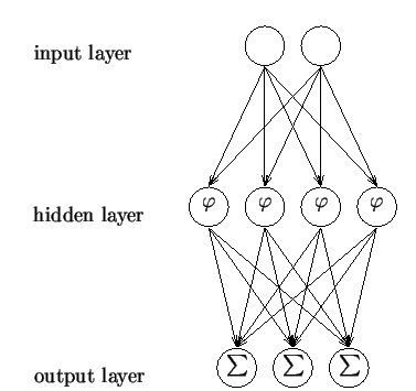
represent a ridge-like function. Below is a graphic representation
of a single-layer perceptron and the one below it is a multi-layer perceptron:


Multi-layer
perceptrons require eight basic elements. A set of processing units,
represented by the circles in the diagram above, a state of activation (is the
unit initially on or off?), and an output function for each unit, which is the
state of activation after the activation rule has been applied. They also need
a pattern of connectivity as represented by the fully connected model above, a
propagation rule which is how information is brought into activations to set
the activation state initially, an activation rule which understands and
manipulates the outputs from the propagation rule, a learning rule which is how
we will train the network, and finally an environment to run it on.
Multi-layer
perceptrons are usually used in “supervised learning” environments, where there
is a training set of input-output pairs that the network must learn to model
and understand. In the perceptron above the training is adapting the weights
and biases accordingly to achieve the desired outcome. To solve the supervised
learning issue in the multi-layer perceptron a “back propagation algorithm” can
be used. A back propagation algorithm has two parts, the forward pass and the
backward pass. The forward pass, the predicted corresponding outputs to the inputs
provided are passed through an equation like the activation function. Then in
the backward pass, partial derivatives of the function with respect to various
parameters are sent back through the network. This process is then iterated
until the weights converge and the error is minimized.
The
Multi-layer perceptron network can also be used for learning that is
unsupervised. This can be done using an “auto-associative structure”. Setting
the same values for both the inputs and outputs of the network creates an
auto-associative structure. The resulting sources will come from the values of
the hidden layer’s units. The network must have at minimum three hidden layers
for any conclusion to be made and it is an incredibly computationally intensive
process.
Rosenblatt’s
discovery of the perceptron revolutionized the world of Artificial Neural
Networks and paved the path for many discoveries in the field and created
countless jobs. He laid the foundation for many artificial intelligence and
pattern recognition software actively used today by large companies like Google
and Facebook.
Helpful Links:


